以下内容均为复制生信菜鸟团的内容,为miRNA-seq的分析教程。
构建miRNA-seq数据分析环境
最近在生信技能树分享了几个miRNA的靶向基因的查询工具,分别是:
很多粉丝留言想听miRNA-seq数据分析流程,主要是上游分析流程,因为下游其实就是表达矩阵分析。跟RNA-seq拿到的counts矩阵是类似的分析策略,只不过是miRNA-seq热度已经过去了,我也仅仅是五年前接触过一次。
其实miRNA-seq数据上游分析有两个方案,一个是仅仅针对已知的miRNA进行定量,这样的话无需比对到物种参考基因组,仅仅是比对到miRNA序列合集即可。另外一个挖掘新的miRNA,主要是考虑到人类对miRNA的认知的不停的进步。当然,如果你想系统性学习,可以参考我五年前在生信菜鸟团自学miRNA-seq分析系列笔记:
- 自学miRNA-seq分析第八讲~miRNA-mRNA表达相关下游分析 | 生信菜鸟团
- 自学miRNA-seq分析第七讲~miRNA样本配对mRNA表达量获取 | 生信菜鸟团
- 自学miRNA-seq分析第六讲~miRNA表达量差异分析 | 生信菜鸟团
- 自学miRNA-seq分析第五讲~miRNA表达量获取 | 生信菜鸟团
- 自学miRNA-seq分析第四讲~测序数据比对 | 生信菜鸟团
- 自学miRNA-seq分析第三讲~公共测序数据下载 | 生信菜鸟团
- 自学miRNA-seq分析第二讲~学习资料的搜集 | 生信菜鸟团
- 自学miRNA-seq分析第一讲~文献选择与解读 | 生信菜鸟团
当然了,如果你是微信阅读,也可以点击:一篇文章学会miRNA-seq分析
首先下载MIRBASE的MIRNA参考序列文件
miRBase是miRNA研究领域最权威的数据库,提供miRNAs序列以及注释查询、定位、发卡序列查询,以及提供命名服务。截止到现在(2020-04-28 ),miRBase 22.1 共收录了271个物种的总共38589 条miRNA信息。其中人类的共收录了1917条pre-miRNA(前体),以及2656条成熟的miRNAs。见:http://www.mirbase.org/
前体miRNA和成熟的miRNA的区别,前体miRNA长度一般是70–120 碱基,一般是茎环结果,也就是发夹结构,所以叫做hairpin。成熟之后,一般22 个碱基。
在 http://www.mirbase.org/ 对应的ftp网站下载如下所示文件:
1 | mkdir -p ~/reference/miRNA |
最后得到的文件如下:
1 | 5.9M Mar 12 2018 hairpin.fa |
构建miRNA-seq数据分析环境只需要使用上面的的文件即可。
然后使用CONDA配置好软件环境
仍然是参考我五年前整理的流程,使用bowtie软件和SHRiMP软件进行比对,然后fastx_toolkit 和fastqc进行质量控制。
1 | conda create -n miRNA |
因为SHRiMP软件太多年没有更新,所以放弃它,反正比对这个过程,有bowtie就ok了。
针对MIRBASE数据库下载的序列构建BOWTIE索引
需要注意的是bowtie和bowtie2不一样哦:
1 | bowtie-build mature.human.fa hsa-mature-bowtie-index |
得到的文件如下:
1 | 4.2M Apr 29 15:42 hsa-hairpin-bowtie-index.1.ebwt |
下载测试数据
这里我们仍然是使用 RNA expression profiling of human iPSC-derived cardiomyocytes in a cardiac hypertrophy model. PLoS One 2014;9(9):e108051. PMID: 25255322 文章里面的 https://www.ncbi.nlm.nih.gov/geo/query/acc.cgi?acc=GSE60292 数据集,如下:
1 | GSM1470353 control-CM, experiment1 |
对应的
1 | SRR1542714 |
仍然是参考:一篇文章学会miRNA-seq分析,简单看看规律
1 | ftp://ftp.sra.ebi.ac.uk/vol1/srr/SRR154/004/SRR1542714; ftp://ftp.sra.ebi.ac.uk/vol1/fastq/SRR154/004/SRR1542714/SRR1542714.fastq.gz |
脚本如下:
1 | mkdir -p ~/reference/miRNA |
得到的sra文件如下:
1 | 33M Apr 29 16:07 SRR1542714.sra |
然后批量转为fq文件, 代码如下:
1 | dump=/home/yb77613/biosoft/sratoolkit/sratoolkit.2.8.2-1-centos_linux64/bin/fastq-dump |
文件如下:
1 | 50M Apr 29 16:14 SRR1542714.fastq.gz |
质控和清洗测序数据
清洗前后,都走一下fastqc图表,清洗主要是fastx_toolkit修剪,代码如下:
1 | ls *gz |while read id |
fastq_quality_filter和fastx_trimmer两个命令,都是来自于fastx_toolkit软件包:
- fastq_quality_filter 代表根据质量过滤序列
- fastx_trimmer 代表缩短FASTQ或FASTQ文件中的读数,根据质量修剪(剪切)序列。
其参数详解如下:
1 | #运行一次查看是否可以成功运行 |
所以 fastq_quality_filter 和 fastx_trimmer命令是有替代品的,就是需要去自行搜索,如果你是要建立好用的miRNA-seq数据分析环境,就需要自己耗费大量时间在里面哦。
最后得到的干净的测序数据文件如下:
1 | 39M Apr 29 16:28 SRR1542714_clean.fq.gz |
前面的步骤,需要自行研究里面的细节哦。
比对 MIRBASE数据库下载的序列 +定量
1 | mature=/home/yb77613/reference/miRNA/hsa-mature-bowtie-index |
使用miRNA序列比对的推荐参数: -n 0 -m1 —best —strata ,理由参考:
对其中一个样本的比对的log日志如下:
1 | SRR1542714_clean.fq.gz |
可以看到,比对率还是蛮低的,但是可以调整参数(允许错配碱基)的数量。
得到的bam文件如下:
1 | 29M Apr 29 20:15 SRR1542714_clean.fq.gz_hairpin.bam |
批量走 samtools idxstats 得到表达量矩阵:
1 | ls *.bam |xargs -i samtools index {} |
比对参考基因组+定量
1 | index=/home/yb77613/reference/index/bowtie/hg38 |
使用默认参数,对其中一个样本的比对的log日志如下:
1 | SRR1542715_clean.fq.gz |
可以看到,这个时候的比对率不得了,得到的bam文件如下:
1 | 34M Apr 29 20:30 SRR1542714_clean.fq.gz_genome.bam |
然后定量,需要使用下面的命令和参数,都是需要看软件文档摸索的。
1 | gtf=/home/yb77613/reference/miRNA/hsa.gff3 |
这样我们就有不同的定量流程拿到的不同的表达矩阵啦。
比较两个定量方式的表达矩阵差异
在featureCounts软件的结果文件 all.counts.id.txt 里面的信息如下:
1 | hsa-miR-12136 chr1 632668 632685 - 18 26 21 50 6 78 19 |
查询其中一个,发现featureCounts软件定量少了80%,比如hsa-miR-12136在featureCounts流程,是 18 26 21 50 6 78 19,但是在miRBase数据库流程,都是五倍以上的表达量。
1 | SRR1542714_clean.fq.gz_matrue.bam.txt:hsa-miR-12136 18 104 0 |
查询另外2个,有意思的是其中一个发现featureCounts软件定量多了1倍,另外一个多了2倍。
1 | SRR1542714_clean.fq.gz_matrue.bam.txt:hsa-miR-34a-5p 22 1745 0 |
比如,hsa-miR-34a-5p在featureCounts流程,是3009 9494 3467 4136 5299 7097,但是在miRBase数据库流程,都只有一半的表达量。
对hsa-miR-34a-3p来说,在featureCounts流程,是88 153 100 86 126 132,但是在miRBase数据库流程,都是两倍的表达量。
这样的定量差异,理论上是不会改变该miRNA的差异分析结果,因为是同样的膨胀系数。
但是,这样的不确定性,让我们的数据分析,蒙上了一层阴影。
文献选择与解读
前些天逛bioStar论坛的时候看到了一个问题,是关于miRNA分析,提问者从NCBI的SRA数据下载文献提供的原始数据,然后处理的时候有些不懂,我看到他列出的数据是iron torrent测序仪的,而且我以前还没玩过miRNA-seq的数据分析, 就抽空自学了一下。因为我有RNA-seq的基础,所以理解学习起来比较简单。特记录一下自己的学习过程,希望对后学者有帮助。
这里选择的文章是2014年发表的,作者用ET-1刺激human iPSCs (hiPSC-CMs) 细胞前后,想看看 miRNA和mRNA表达量的变化,我并没有细看该文章的生物学意义,仅仅从数据分析的角度解读一下这篇文章,mRNA表达量用的是Affymetrix Human Genome U133 Plus 2.0 Array,分析起来特别容易,就是得到表达矩阵,然后用limma这个包找找差异表达基因即可。但是mRNA分析起来就有点麻烦了,作者用的是iron torrent测序仪,但是从SRA数据中心下载的是已经去掉接头的测序数据,fastq格式的,所以这里其实并不需要考虑测序仪的特异性。
关于该文章的几个资料收集如下:
## paper : http://journals.plos.org/plosone/article?id=10.1371/journal.pone.0108051
## Aggarwal P, Turner A, Matter A, Kattman SJ et al. RNA expression profiling of human iPSC-derived cardiomyocytes in a cardiac hypertrophy model. PLoS One 2014;9(9):e108051. PMID: 25255322
## The accession numbers are 1. SuperSeries (mRNA+miRNA) - GSE60293
## 2. mRNA expression array - GSE60291 (Affymetrix Human Genome U133 Plus 2.0 Array)
## 3. miRNA-Seq - GSE60292 (Ion Torrent)
## GEO : http://www.ncbi.nlm.nih.gov/geo/query/acc.cgi?acc=GSE60292
## FTP : ftp://ftp-trace.ncbi.nlm.nih.gov/sra/sra-instant/reads/ByStudy/sra/SRP/SRP045/SRP045420
仔细看看该文章做了哪些分析,然后才能自己模仿,得到同样的数据分析结果。
该文章处理数据的流程是:
Ion Torrent’s Torrent Suite version 3.6 was used for basecalling
Raw sequencing reads were aligned using the SHRiMP2 aligner and were aligned against the human reference genome (hg19) for novel miRNA prediction and then against a custom reference sequence file containing miRBase v.20 known human miRNA hairpins, tRNA, rRNA, adapter sequences and predicted novel miRNA sequences.(Genome_build: hg19, miRBase v.20 human miRNA hairpins)
The miRDeep2 package (default parameters) was used to predict novel (as yet undescribed) miRNAs
Alignments with less than 17 bp matches and a custom 3′ end phred q-score threshold of 17 were filtered out.
miRNA quanitification was done using HTSeq v0.5.3p3 using the default union parameter.
Differential miRNA expression was analyzed using the DESeq (v.1.12.1) R/Bioconductor package
In this study, differentially expressed genes that had a false discovery rate cutoff at 10% (FDR< = 0.1), a log2 fold change greater than 1.5 and less than −1.5 were considered significant.
Target gene prediction was performed using the TargetScan (version 6.2) database
We also used miRTarBase (version 4.3), to identify targets that have been experimentally validated
## miR-Deep2 and miReap ## predict exact precursor sequence according from mature sequence
文章提到了fastq数据质量控制标准,数据比对工具,比对的参考基因组(两条比对线路),miRNA表达量的得到,新的miRNA预测,miRNA靶基因预测,这也是我们学习miRNA-seq的数据分析的标准套路, 而且作者给出了所有的分析结果,我们完全可以通过自己的学习来重现他的分析过程。
Supplementary_files_format_and_content: tab-delimited text files containing raw read counts for known mature human miRNAs.(表达矩阵)
We detected 836 known human mature miRNAs in the control-CMs and 769 in the ET1-CMs
Based on our miRNA-Seq data, we predicted 506 sequences to be potentially novel, as yet undescribed miRNAs.
In order to validate the expression profiles of the miRNAs detected, we performed RT-qPCR on a subset of five known human mature and five of our predicted novel miRNAs.
we obtained a total of 1,922 predicted miRNA-mRNA pairs represented by 309 genes and 174 known mature human miRNAs. ()
当然仅仅是套路分析无法发文章的,所以他结合了 miRNA和mRNA 进行网络分析,还做了少量湿实验来验证,最后还扯了一些生物学意义,当然这种纯粹理论分析肯定不好扯什么治病救人的伟大理想。
学习资料的搜集
因为我也是完全从零开始入门miRNA-seq分析,所以收集的资料比较齐全,我首先看了部分中文资料,了解了miRNA测序是怎么回事,该分析什么,然后主要围绕着上一篇提到的文献里面的分析步骤来搜索资料。传送门:自学miRNA-seq分析第一讲~文献选择与解
我首先拿到了miRNA定义:http://nar.oxfordjournals.org/content/34/suppl_1/D135.full ,当然基本上每个研究miRNA的文章都会在前言里面写到这个,我只是随意列出一个而已。
MicroRNAs (miRNAs) are small RNA molecules, which are ∼22 nt sequences that have an important role in the translational regulation and degradation of mRNA by the base’s pairing to the 3′-untranslated regions (3′-UTR) of the mRNAs. The miRNAs are derived from the precursor transcripts of ∼70–120 nt sequences, which fold to form as stem–loop structures, which are thought to be highly conserved in the evolution of genomes. Previous analyses have suggested that ∼1% of all human genes are miRNA genes, which regulate the production of protein for 10% or more of all human coding genes。
然后我比较纠结的问题是参考序列如何选择,因为miRNA序列很少,把它map到3G大小的人类基因组有点浪费计算资源,正好我的服务器又坏了,不想太麻烦,想用自己的个人电脑搞定这个学习过程。我看到很多帖子提到的都是比对到参考miRNA数据库(miRNA count: 28645 entries),用bowtie : http://www.mirbase.org/ ,从这个数据库,我明白了前体miRNA和成熟的miRNA的区别,前体miRNA长度一般是∼70–120 碱基,前体miRNA一般是茎环结果,也就是发夹结构,所以叫做hairpin。成熟之后,一般∼22 个碱基,在miRNA数据库很容易下载到这些数据,现在的miRNA版本来说,人类这个物种已知的成熟miRNA共有2588条序列,而前体miRNA共有1881条序列,我下载(下载时间2016年6月 )的代码是:
wget ftp://mirbase.org/pub/mirbase/CURRENT/hairpin.fa.gz ## 28645 reads
wget ftp://mirbase.org/pub/mirbase/CURRENT/mature.fa.zip ## 35828 reads
wget ftp://mirbase.org/pub/mirbase/CURRENT/hairpin.fa.zip
wget ftp://mirbase.org/pub/mirbase/CURRENT/genomes/hsa.gff3 ##
wget ftp://mirbase.org/pub/mirbase/CURRENT/miFam.dat.zipgrep sapiens mature.fa |wc # 2588
grep sapiens hairpin.fa |wc # 1881
## Homo sapiens
perl -alne ‘{if(/^>/){if(/Homo/){$tmp=1}else{$tmp=0}};next if $tmp!=1;s/U/T/g if !/>/;print }’ hairpin.fa >hairpin.human.fa
perl -alne ‘{if(/^>/){if(/Homo/){$tmp=1}else{$tmp=0}};next if $tmp!=1;s/U/T/g if !/>/;print }’ mature.fa >mature.human.fa
这里值得一提的是miRBase数据库下载的序列,居然都是用U表示的,也就是说就是miRNA序列,而不是转录成该miRNA的基因序列,而我们测序的都是基因序列。
通过这个代码制作的 hairpin.human.fa 和 mature.human.fa 就是本次数据分析的参考基因组。
搜集资料的过程中,我看到了一篇文献讲挖掘1000genomes的数据找到位于miRNA的snp位点,https://genomemedicine.biomedcentral.com/articles/10.1186/gm363 ,看起来比较新奇,不过跟本次学习过程没有关系,我就是记录一下,有空回来学习学习。
同时,我看到了一些博客讲解如何分析miRNA数据:http://genomespot.blogspot.com/2013/08/quick-alignment-of-microrna-seq-data-to.html
还有很多公司讲数据分析流程:
http://bioinfo5.ugr.es/miRanalyzer/miRanalyzer_tutorial.html
http://www.partek.com/sites/default/files/Assets/UserGuideMicroRNAPipeline.pdf
http://partek.com/Tutorials/microarray/microRNA/miRNA_tutorial.pdf
http://www.arraystar.com/reviews/microrna-sequencing-data-analysis-guideline/
http://bioinfo5.ugr.es/sRNAbench/sRNAbench_tutorial.pdf
http://seqcluster.readthedocs.io/mirna_annotation.html
耶鲁大学好像做得不错: http://www.yale.edu/giraldezlab/miRNA.html
中国有个南方基因: http://www.southgene.com/newsshow.php?cid=55&id=73
miRNA研究整套方案 http://wenku.baidu.com/view/5f38577a31b765ce05081429.html?re=view
Biostar 讨论帖子:
https://www.biostars.org/p/3344/
https://www.biostars.org/p/98486/
miRNA-seq数据处理实战指南: http://bib.oxfordjournals.org/content/early/2015/04/17/bib.bbv019.full
直接用一个包也可以搞定: http://bioconductor.org/packages/release/bioc/html/easyRNASeq.html
github流程:miRNA Analysis Pipeline v0.2.7 https://github.com/bcgsc/mirna/tree/master/v0.2.7
https://tools.thermofisher.com/content/sfs/manuals/CO25176_0512.pdf
miRNA annotation : http://seqcluster.readthedocs.io/mirna_annotation.html
开发的网页版分析工具: https://wiki.uio.no/projects/clsi/images/2/2f/HTS_2014_miRNA_analysis_Lifeportal_14_final.pdf
R package 也很好用: http://bioinf.wehi.edu.au/subread-package/SubreadUsersGuide.pdf
一个培训: http://www.training.prace-ri.eu/uploads/tx_pracetmo/NGSdataAnalysisWithChipster.pdf
可视化IGV User Guide: http://www.broadinstitute.org/igv/book/export/html/6
比较特殊的是新的miRNA预测,miRNA靶基因预测,这块研究太多软件了,并没有成型的流程和标准。
公共测序数据下载
前面已经讲到了该文章的数据已经上传到NCBI的SRA数据中心,所以直接根据索引号下载,然后用SRAtoolkit转出我们想要的fastq测序数据即可。下载的数据一般要进行质量控制,可视化展现一下质量如何,然后根据大题测序质量进行简单过滤。所以需要提前安装一些软件来完成这些任务,包括: sratoolkit /fastx_toolkit /fastqc/bowtie2/hg19/miRBase/SHRiMP
下面是我用新服务器下载安装软件的一些代码记录,因为fastx_toolkit /fastqc我已经安装过,就不列代码了,还有miRBase的下载,我在前面第二讲里面提到过,传送门:自学miRNA-seq分析第二讲~学习资料的搜集
## pre-step: download sratoolkit /fastx_toolkit_0.0.13/fastqc/bowtie2/hg19/miRBase/SHRiMP
## http://www.ncbi.nlm.nih.gov/Traces/sra/sra.cgi?view=software
## http://www.ncbi.nlm.nih.gov/books/NBK158900/
## 我这里特意挑选的二进制版本程序下载的,这样直接解压就可以用,但是需要挑选适合自己的操作系统的程序。
cd ~/biosoft
mkdir sratoolkit && cd sratoolkit
wget http://ftp-trace.ncbi.nlm.nih.gov/sra/sdk/2.6.3/sratoolkit.2.6.3-centos_linux64.tar.gz
##
## Length: 63453761 (61M) [application/x-gzip]
## Saving to: “sratoolkit.2.6.3-centos_linux64.tar.gz”
tar zxvf sratoolkit.2.6.3-centos_linux64.tar.gz
cd ~/biosoft
mkdir bowtie && cd bowtie
wget https://sourceforge.net/projects/bowtie-bio/files/bowtie2/2.2.9/bowtie2-2.2.9-linux-x86_64.zip/download#Length: 27073243 (26M) [application/octet-stream]
#Saving to: “download”
mv download bowtie2-2.2.9-linux-x86_64.zip
unzip bowtie2-2.2.9-linux-x86_64.zip
## http://compbio.cs.toronto.edu/shrimp/
mkdir SHRiMP && cd SHRiMP
wget http://compbio.cs.toronto.edu/shrimp/releases/SHRiMP_2_2_3.lx26.x86_64.tar.gz
tar zxvf SHRiMP_2_2_3.lx26.x86_64.tar.gz
cd SHRiMP_2_2_3
export SHRIMP_FOLDER=$PWD ## 这个软件使用的时候比较奇葩,需要设置到环境变量,不能简单的调用全路径
SHRiMP这个软件比较小众,我也是第一次听说过,本来我计划是能用bowtie搞定,就不麻烦了,但是第一次比对出了一个bug,就是下载的miRNA序列里面的U没有转换成T,所以导致比对率非常之低,所以我不得不根据文章里面记录的软件SHRiMP 来做比对,最后发现比对率完全没有改善,搞得我都在怀疑是不是作者乱来了。
下面是下载数据,质量控制的代码,希望大家可以照着运行一下:
## step1 : download raw data
mkdir miRNAtest && cd miRNA_test
echo {14..19} |sed ‘s/ /\n/g’ |while read id; \
do wget “ftp://ftp-trace.ncbi.nlm.nih.gov/sra/sra-instant/reads/ByStudy/sra/SRP/SRP045/SRP045420/SRR15427$id/SRR15427$id.sra“ ;\
done
## step2 : change sra data to fastq files.
## 主要是用shell脚本来批量下载
ls sra |while read id; do ~/biosoft/sratoolkit/sratoolkit.2.6.3-centos_linux64/bin/fastq-dump $id;done
rm sra
## 33M —> 247M
#Read 1866654 spots for SRR1542714.sra
#Written 1866654 spots for SRR1542714.sra
## step3 : download the results from paper
## http://www.bio-info-trainee.com/1571.html
## ftp://ftp.ncbi.nlm.nih.gov/geo/series/GSE1nnn/GSE1009/suppl/GSE1009_RAW.tar
mkdir paper_results && cd paper_results
wget ftp://ftp.ncbi.nlm.nih.gov/geo/series/GSE60nnn/GSE60292/suppl/GSE60292_RAW.tar
## tar xvf GSE60292_RAW.tar
ls *gz |while read id ; do (echo $id;zcat $id | cut -f 2 |perl -alne ‘{$t+=$;}END{print $t}’);done
ls gz |xargs gunzip
## step4 : quality assessment
ls fastq | while read id ; do ~/biosoft/fastqc/FastQC/fastqc $id;done
## Sequence length 8-109
## %GC 52
## Adapter Content passed
## write a script : :: cat >filter.sh
ls fastq |while read id
do
echo $id
~/biosoft/fastx_toolkit_0.0.13/bin/fastq_quality_filter -v -q 20 -p 80 -Q33 -i $id -o tmp ;
~/biosoft/fastx_toolkit_0.0.13/bin/fastx_trimmer -v -f 1 -l 27 -i tmp -Q33 -z -o ${id%%.}_clean.fq.gz ;
done
rm tmp
## discarded 12%~~49%%
ls _clean.fq.gz | while read id ; do ~/biosoft/fastqc/FastQC/fastqc $id;done
mkdir QC_results
mv zip *html QC_results
这个代码是我自己根据文章的理解写出的,因为我本身不擅长miRNA数据分析,所以在进行QC的时候参数选择可能并不是那么友好,如果有高手能指正就最好了,可以直接打我电话告诉我,或者发邮箱给我,邮箱用户名是jmzeng1314,是163邮箱。
~/biosoft/fastx_toolkit_0.0.13/bin/fastq_quality_filter -v -q 20 -p 80 -Q33 -i $id -o tmp ;
~/biosoft/fastx_toolkit_0.0.13/bin/fastx_trimmer -v -f 1 -l 27 -i tmp -Q33 -z -o ${id%%.*}_clean.fq.gz ;
最后得到的clean.fq.gz系列文件,就是我需要进行比对的序列啦。
测序数据比对
序列比对是大多数类型数据分析的核心,如果要利用好测序数据,比对细节非常重要,我这里只是研读一篇文章也就没有对比对细节过多考虑,只是列出自己的代码和自己的几点思考,力求重现文章作者的分析结果。对miRNA-seq数据有两条比对策略,一种是下载miRBase数据库里面的已知miRNA序列来进行比对,一种直接比对到参考基因组(比如人类的是hg19/hg38),前面的比对非常简单,而且很容易就可以数出已经的所以miRNA序列的表达量,后面的比对有点耗时,而且算表达量的时候也不是很方便,但是它有个有点是可以来预测新的miRNA,所以大多数文章都会把这两条路给走一下。
本文选择的是SHRiMP这个小众软件,起初我并没有在意,就用的bowtie2而已,参考基因组我这里因为服务器原因,就用了miRBase数据库下载的人类的参考序列,现在的miRNA版本来说,人类这个物种已知的成熟miRNA共有2588条序列,而前体miRNA共有1881条序列,我下载(下载时间2016年6月 )的代码见 自学miRNA-seq分析第二讲~学习资料的搜集 ,下面比对所用到的软件已经序列在我的: 自学miRNA-seq分析第三讲~公共测序数据下载
## step5 : alignment to miRBase v21 (hairpin.human.fa/mature.human.fa )
#### step5.1 using bowtie2 to do alignment
mkdir bowtie2_index && cd bowtie2_index
~/biosoft/bowtie/bowtie2-2.2.9/bowtie2-build ../hairpin.human.fa hairpin_human
~/biosoft/bowtie/bowtie2-2.2.9/bowtie2-build ../mature.human.fa mature_human
ls _clean.fq.gz | while read id ; do ~/biosoft/bowtie/bowtie2-2.2.9/bowtie2 -x miRBase/bowtie2_index/hairpin_human -U $id -S ${id%%.}.hairpin.sam ; done
## overall alignment rate: 10.20% / 5.71%/ 10.18%/ 4.36% / 10.02% / 4.95% (before convert U to T )
## overall alignment rate: 51.77% / 70.38%/51.45% /61.14%/ 52.20% / 65.85% (after convert U to T )
ls _clean.fq.gz | while read id ; do ~/biosoft/bowtie/bowtie2-2.2.9/bowtie2 -x miRBase/bowtie2_index/mature_human -U $id -S ${id%%.}.mature.sam ; done
## overall alignment rate: 6.67% / 3.78% / 6.70% / 2.80%/ 6.55% / 3.23% (before convert U to T )
## overall alignment rate: 34.94% / 46.16%/ 35.00%/ 38.50% / 35.46% /42.41%(after convert U to T )
#### step5.2 using SHRiMP to do alignment
## http://compbio.cs.toronto.edu/shrimp/README
## 3.5 Mapping cDNA reads against a miRNA database
cd ~/biosoft/SHRiMP/SHRiMP_2_2_3
export SHRIMP_FOLDER=$PWD
cd -
## We project the database with:
$SHRIMP_FOLDER/utils/project-db.py —seed 00111111001111111100,00111111110011111100,00111111111100111100,00111111111111001100,00111111111111110000 \
—h-flag —shrimp-mode ls miRBase/hairpin.human.fa
##
$SHRIMP_FOLDER/bin/gmapper-ls -L hairpin.human-ls SRR1542716.fastq —qv-offset 33 \
-o 1 -H -E -a -1 -q -30 -g -30 —qv-offset 33 —strata -N 8 >map.out 2>map.log
大家可以看到我们把测序reads比对到前体miRNA和成熟的miRNA结果是有略微区别的,因为一个前体miRNA可以形成多个成熟的miRNA,而并不是所有的成熟的miRNA形式都被记录在数据库,所以一般推荐我们比对到前体miRNA数据库,这样还可以预测新的成熟miRNA,也是非常有意义的。
而且有个非常重要的一点,就是大家可以看到我把U变成T前后比对率差异非常大,这其实是一个非常蠢的错误。我就不多说了。但是做到这一步,其实可以跟文章来做验证了,文章有提到比对率,比对的序列。
我也是在博客里面看到这个信息的:
Thank you so much!. Yes I contacted the lab-guy and he just said that trimmed the first 4 bp and last 4bp. ( as you found)
So I firstly trimmed the adapter sequences(TGGAATTCTCGGGTGCCAAGGAACTCCAGTCAC)
And then, trimmed the first 4bp and last 4bp from reads, which leads to the 22bp peak of read-length distribution(instead of 24bp)
Anyhow, I tried to map with bowtie2 again.
> bowtie2 —local -N 1 -L 16
-x ../miRNA_reference/hairpin_UtoT.fa
-U first4bptrimmed_A1-SmallRNA_S1_L001_R1_001_Illuminaadpatertrim.fastq
-S f4_trimmed.sam
I also changed hairpin.fa file (U to T)
Oh.. thank you David,
Finallly, I got
2565353 reads; of these:
2565353 (100.00%) were unpaired; of these:
479292 (18.68%) aligned 0 times
11959 (0.47%) aligned exactly 1 time
2074102 (80.85%) aligned >1 times
81.32% overall alignment rate
miRNA表达量获取
拿到比对后的sam/bam文件之后,这只能算是level2的数据,一般我们给他人share我们的结果也是直接给表达矩阵的, miRNA分析跟mRNA分析类似,但是它的表达矩阵更好获取一点。如果是mRNA,我们一般会跟基因组来比较,而基因组就那24条参考染色体,想知道具体比对到了哪个基因,需要根据基因组注释文件来写程序提取表达量信息,现在比较流行的是htseq这个软件,我前面也写过教程如何安装和使用,这里就不啰嗦了。但是对于miRNA,因为我比对的就是那1881条前体miRNA序列,所以直接分析比对的sam/bam文件就可以知道每条参考miRNA序列的表达量了。
## step6: counts the reads which mapping to each miRNA reference.
## we need to exclude unmapped as well as multiple-mapped reads
## XS:i:Alignment score for second-best alignment. Can be negative. Can be greater than 0 in —local mode
## NM:i:1 ## NM i Edit distance to the reference, including ambiguous bases but excluding clipping
#The following command exclude unmapped (-F 4) as well as multiple-mapped (grep -v “XS:”) reads
#samtools view -F 4 input.bam | grep -v “XS:” | wc -l
## 180466//1520320
##cat >count.hairpin.sh
ls hairpin.sam | while read id
do
**samtools view -SF 4 $id |perl -alne ‘{$h{$F[2]}++}END{print “$\t$h{$}” foreach sort keys %h }’ > ${id%%_\}.hairpin.counts
done
## bash count.hairpin.sh
##cat >count.mature.sh
ls *mature.sam | while read id
do samtools view -SF 4 $id |perl -alne ‘{$h{$F[2]}++}END{print “$\t$h{$}” foreach sort keys %h }’ > ${id%%_*}.mature.counts**
done
## bash count.mature.sh
上面的代码,是我自己写的脚本来算表达量,非常简单,因为我没有考虑细节,直接想得到各个样本测序数据的表达量而已。如果是比对到了参考基因组,就要根据miRNA的gff注释文件用htseq等软件来计算表达量啦。
得到了表达量,就可以跟文献来做比较啦:
### step7: compare the results with paper’s
GSM1470353: control-CM, experiment1; Homo sapiens; miRNA-Seq SRR1542714
GSM1470354: ET1-CM, experiment1; Homo sapiens; miRNA-Seq SRR1542715
GSM1470355: control-CM, experiment2; Homo sapiens; miRNA-SeqSRR1542716
GSM1470356: ET1-CM, experiment2; Homo sapiens; miRNA-Seq SRR1542717
GSM1470357: control-CM, experiment3; Homo sapiens; miRNA-Seq SRR1542718
GSM1470358: ET1-CM, experiment3; Homo sapiens; miRNA-Seq SRR1542719
### 下面我用R语言来检验一下,我得到的分析结果跟文章发表的结果的区别。
a=read.table(“bowtie_bam/SRR1542714.mature.counts”)
b=read.table(“paper_results/GSM1470353_iPS_010313_Unstim_known_miRNA_counts.txt”)
plot(log(tmp[,2]),log(tmp[,3]))
cor(tmp[,2],tmp[,3])
##[1] 0.8413439
miRNA表达量差异分析
这一讲是miRNA-seq数据分析的分水岭,前面的5讲说的是读文献下载数据比对然后计算表达量,属于常规的流程分析,一般在公司测序之后都可以拿到分析结果,或者文献也会给出下载结果。但是单纯的分析一个样本意义不大,一般来说,我们做研究都是针对于不同状态下的miRNA表达量差异分析,然后做注释,功能分析,网络分析,这才是重点,也是难点。我这里就直接拿文献处理好的miRNA表达量来展示如何做下游分析,首先就是差异分析啦:根据文献,我们可以知道样本的分类情况是:
GSM1470353: control-CM, experiment1; Homo sapiens; miRNA-Seq SRR1542714
GSM1470354: ET1-CM, experiment1; Homo sapiens; miRNA-Seq SRR1542715
GSM1470355: control-CM, experiment2; Homo sapiens; miRNA-SeqSRR1542716
GSM1470356: ET1-CM, experiment2; Homo sapiens; miRNA-Seq SRR1542717
GSM1470357: control-CM, experiment3; Homo sapiens; miRNA-Seq SRR1542718
GSM1470358: ET1-CM, experiment3; Homo sapiens; miRNA-Seq SRR1542719
可以看到是6个样本的测序数据,分成两组,就是ET1刺激了CM细胞系前后对比而已!
同时,我们也拿到了这6个样本的表达矩阵,计量单位是counts的reads数,所以我们一般会选用DESeq2,edgeR这样的常用包来做差异分析,当然,做差异分析的工具还有十几个,我这里只是拿一根最顺手的举例子,就是DESeq2
下面的代码有点长,因为我在bioconductor系列教程里面多次提到了DESeq2使用方法,这里就只贴出代码,反正我要说的重点就是,我们进行了差异分析,然后得到差异miRNA列表
### step8: differential expression analysis by R package for miRNA expression patterns:
## 文章里面提到的结果是:
MicroRNA sequencing revealed over 250 known and 34 predicted novel miRNAs to be differentially expressed between ET-1 stimulated and unstimulated control hiPSC-CMs.
## (FDR < 0.1 and 1.5 fold change)
rm(list=ls())
setwd(‘J:\miRNAtest\paper_results’) ##把从GEO里面下载的文献结果放在这里
sampleIDs=c()
groupList=c()
allFiles=list.files(pattern = ‘.txt’)
i=allFiles[1]
sampleID=strsplit(i,”“)[[1]][1]
treat=strsplit(i,”“)[[1]][4]
dat=read.table(i,stringsAsFactors = F)
colnames(dat)=c(‘miRNA’,sampleID)
groupList=c(groupList,treat)
for (i in allFiles[-1]){
sampleID=strsplit(i,”“)[[1]][1]
treat=strsplit(i,”_”)[[1]][4]
a=read.table(i,stringsAsFactors = F)
colnames(a)=c(‘miRNA’,sampleID)
dat=merge(dat,a,by=’miRNA’)
groupList=c(groupList,treat)
}
### 上面的代码只是为了把6个独立的表达文件给合并成一个表达矩阵
## we need to filter the low expression level miRNA
exprSet=dat[,-1]
rownames(exprSet)=dat[,1]
suppressMessages(library(DESeq2))
exprSet=ceiling(exprSet)
(colData <- data.frame(row.names=colnames(exprSet), groupList=groupList))## DESeq2就是这么简单的用
dds <- DESeqDataSetFromMatrix(countData = exprSet,
colData = colData,
design = ~ groupList)
dds <- DESeq(dds)
png(“qc_dispersions.png”, 1000, 1000, pointsize=20)
plotDispEsts(dds, main=”Dispersion plot”)
dev.off()
res <- results(dds)
## 画一些图,相当于做QC吧
png(“RAWvsNORM.png”)
rld <- rlogTransformation(dds)
exprSet_new=assay(rld)
par(cex = 0.7)
n.sample=ncol(exprSet)
if(n.sample>40) par(cex = 0.5)
cols <- rainbow(n.sample*1.2)
par(mfrow=c(2,2))
boxplot(exprSet, col = cols,main=”expression value”,las=2)
boxplot(exprSet_new, col = cols,main=”expression value”,las=2)
hist(exprSet[,1])
hist(exprSet_new[,1])
dev.off()library(RColorBrewer)
(mycols <- brewer.pal(8, “Dark2”)[1:length(unique(groupList))])# Sample distance heatmap
sampleDists <- as.matrix(dist(t(exprSet_new)))
#install.packages(“gplots”,repos = “http://cran.us.r-project.org“)
library(gplots)
png(“qc-heatmap-samples.png”, w=1000, h=1000, pointsize=20)
heatmap.2(as.matrix(sampleDists), key=F, trace=”none”,
col=colorpanel(100, “black”, “white”),
ColSideColors=mycols[groupList], RowSideColors=mycols[groupList],
margin=c(10, 10), main=”Sample Distance Matrix”)
dev.off()png(“MA.png”)
DESeq2::plotMA(res, main=”DESeq2”, ylim=c(-2,2))
dev.off()
## 重点就是这里啦,得到了差异分析的结果
resOrdered <- res[order(res$padj),]
resOrdered=as.data.frame(resOrdered)
write.csv(resOrdered,”deseq2.results.csv“,quote = F)##下面也是一些图,主要是看看样本之间的差异情况
library(limma)
plotMDS(log(counts(dds, normalized=TRUE) + 1))
plotMDS(log(counts(dds, normalized=TRUE) + 1) - log(t( t(assays(dds)[[“mu”]]) / sizeFactors(dds) ) + 1))
plotMDS( assays(dds)[[“counts”]] ) ## raw count
plotMDS( assays(dds)[[“mu”]] ) ##- fitted values.
最后我们得到的差异分析结果:deseq2.results.csv,就可以跟进FDR和fold change来挑选符合要求的差异miRNA啦
miRNA样本配对mRNA表达量获取
这一讲其实算不上是自学miRNA-seq分析,本质就是affymetrix的mRNA表达芯片数据分析,而且还是最常用的那种GPL570 HG-U133_Plus_2,但是因为是跟miRNA样本配对检测的,而且后面会利用到这两个数据分析结果来做共表达网络分析等等,所以就贴出对该芯片数据的分析结果。文章里面也提到了 Messenger RNA expression analysis identified 731 probe sets with significant differential expression,作者挑选的差异分析结果的显著基因列表如下:## http://journals.plos.org/plosone/article/asset?unique&id=info:doi/10.1371/journal.pone.0108051.s002
## mRNA expression array - GSE60291 (Affymetrix Human Genome U133 Plus 2.0 Array)
hgu133plus2芯片数据太常见了,可以从GEO里面下载该study的原始测序数据,然后用affy,limma包来分析,也可以直接用GEOquery包来下载作者分析好的表达矩阵,然后直接做差异分析。我这里选择的是后者,而且我跟作者分析方法有一点区别是,我先把探针都注释好了基因,然后对每个基因只挑最大表达量的基因。而作者是直接对探针为单位的的表达矩阵进行差异分析,对分析结果里面的探针进行基因注释。我这里无法给出哪种方法好的绝对评价。代码如下:
rm(list=ls())
library(GEOquery)
library(limma)
GSE60291 <- getGEO(‘GSE60291’, destdir=”.”,getGPL = F)#下面是表达矩阵
exprSet=exprs(GSE60291[[1]])
library(“annotate”)
GSE60291[[1]]
## 下面是分组信息
pdata=pData(GSE60291[[1]])
treatment=factor(unlist(lapply(pdata$title,function(x) strsplit(as.character(x),”-“)[[1]][1])))
#treatment=relevel(treatment,’control’)
## 下面做基因注释
platformDB=’hgu133plus2.db’
library(platformDB, character.only=TRUE)
probeset <- featureNames(GSE60291[[1]])
#EGID <- as.numeric(lookUp(probeset, platformDB, “ENTREZID”))
SYMBOL <- lookUp(probeset, platformDB, “SYMBOL”)
## 下面对每个基因挑选最大表达量探针
a=cbind(SYMBOL,exprSet)
## remove the duplicated probeset
rmDupID <-function(a=matrix(c(1,1:5,2,2:6,2,3:7),ncol=6)){
exprSet=a[,-1]
rowMeans=apply(exprSet,1,function(x) mean(as.numeric(x),na.rm=T))
a=a[order(rowMeans,decreasing=T),]
exprSet=a[!duplicated(a[,1]),]
#
exprSet=exprSet[!is.na(exprSet[,1]),]
rownames(exprSet)=exprSet[,1]
exprSet=exprSet[,-1]
return(exprSet)
}
exprSet=rmDupID(a)
rn=rownames(exprSet)
exprSet=apply(exprSet,2,as.numeric)
rownames(exprSet)=rn
exprSet[1:4,1:4]
#exprSet=log(exprSet) ## based on e
boxplot(exprSet,las=2)
## 下面用limma包来进行芯片数据差异分析
design=model.matrix(~ treatment)
fit=lmFit(exprSet,design)
fit=eBayes(fit)
#vennDiagram(decideTests(fit))
DEG=topTable(fit,coef=2,n=Inf,adjust=’BH’)
dim(DEG[abs(DEG[,1])>1.2 & DEG[,5]<0.05,]) ## 806 genes
write.csv(DEG,”ET1-normal.DEG.csv”)
得到的ET1-normal.DEG.csv 文件就是我们的差异分析结果,可以跟文章提供的差异结果做比较,是几乎一模一样的!
如果根据logFC 1.2 p 矫正P 值0.05来挑选,可以拿到806个基因。
miRNA-mRNA表达相关下游分析
通过前面的分析,我们已经量化了ET1刺激前后的细胞的miRNA和mRNA表达水平,也通过成熟的统计学分析分别得到了差异miRNA和mRNA,这时候我们就需要换一个参考文献了,因为前面提到的那篇文章分析的不够细致,我这里选择了浙江大学的一篇TCGA数据挖掘分析文章Identifying miRNA/mRNA negative regulation pairs in colorectal cancer,里面首先就是查找miRNA-mRNA基因对,因为miRNA主要还是负向调控mRNA表达,所以根据我们得到的两个表达矩阵做相关性分析,很容易得到符合统计学意义的miRNA-mRNA基因对,具体分析内容如下:
把得到的差异miRNA的表达量画一个热图,看看它是否能显著的分类
用miRWalk2.0等数据库或者根据来获取这些差异miRNA的validated target genes
然后看看这些pairs of miRNA- target genes的表达量相关系数,选取显著正相关或者负相关的pairs
这些被选取的pairs of miRNA- target genes拿去做富集分析
最后这些pairs of miRNA- target genes做PPI网络分析
首先我们看第一个热图的实现:
resOrdered=na.omit(resOrdered)
DEmiRNA=resOrdered[abs(resOrdered$log2FoldChange)>log2(1.5) & resOrdered$padj <0.01 ,]
write.csv(resOrdered,”deseq2.results.csv”,quote = F)
DEmiRNAexprSet=exprSet[rownames(DEmiRNA),]
write.csv(DEmiRNAexprSet,’DEmiRNAexprSet.csv’)DEmiRNAexprSet=read.csv(‘DEmiRNAexprSet.csv‘,stringsAsFactors = F)
exprSet=as.matrix(DEmiRNAexprSet[,2:7])
rownames(exprSet)=rownames(DEmiRNAexprSet)
heatmap(exprSet)
gplots::heatmap.2(exprSet)
library(pheatmap)
## http://biit.cs.ut.ee/clustvis/
因为我前面保存的表达量就基于counts的,所以画热图还需要进行normalization,我这里懒得弄了,就用了一个网页版工具,自动出热图http://biit.cs.ut.ee/clustvis/
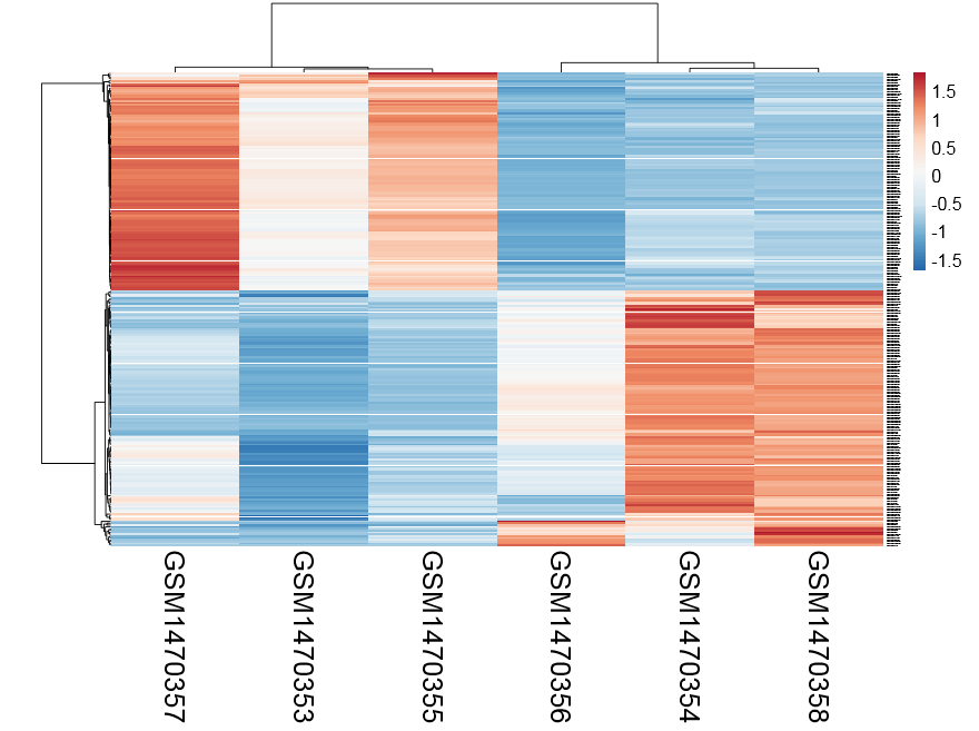
感觉还不错,可以很清楚的看到ET1刺激前后细胞中miRNA表达量变化
然后就是检验我们选取的感兴趣的有显著差异的miRNA的target genes,这时候有两种方法,一个是先由数据库得到已经被检验的miRNA的target genes,另一种是根据miRNA和mRNA表达量的相关性来预测。
用数据库来查找MiRNA的作用基因,非常多的工具,比较常用的有TargetScan/miRTarBase
### http://nar.oxfordjournals.org/content/early/2015/11/19/nar.gkv1258.full
### http://mirtarbase.mbc.nctu.edu.tw/
### http://mirtarbase.mbc.nctu.edu.tw/cache/download/6.1/hsa_MTI.xlsx
### http://www.targetscan.org/vert_71/ (version 7.1 (June 2016))
我还看到过一个整合工具: miRecords (DIANA-microT, MicroInspector, miRanda, MirTarget2, miTarget, NBmiRTar, PicTar, PITA, RNA22, RNAhybrid and TargetScan/TargertScanS)里面提到了查找MiRNA的作用基因这一过程,高假阳性,至少被5种工具支持,才算是真的
还有很多类似的工具,miRWalk2,psRNATarget网页版工具,最后值得一提的是中山大学的: starBase Pan-Cancer Analysis Platform is designed for deciphering Pan-Cancer Networks of lncRNAs, miRNAs, ceRNAs and RNA-binding proteins (RBPs) by mining clinical and expression profiles of 14 cancer types (>6000 samples) from The Cancer Genome Atlas (TCGA) Data Portal (all data available without limitations).虽然我没有仔细的用,但是看介绍好牛的样子,还有一个R包:miRLAB我玩了一会,它是先通过算所有配对的miRNA- genes的表达量相关系数,选取显著正相关或者负相关的pairs,然后反过来通过已知数据库来验证。
后面我就不讲了,主要看你得到miRNA的时候其它生物学数据是否充分,如果是癌症病人,有生存相关数据,可以做生存分析,如果你同时测了甲基化数据,可以做甲基化相关分析~~~~~
如果只是单纯的miRNA测序数据,可以回过头去研究一下de novo的miRNA预测的步骤,也是研究重点
引用
参考文章如引起任何侵权问题,可以与我联系,谢谢。